Using AI Agents for a Distributor’s Demand Forecasting

Most forecasting problems are relatively stable. A few things make it brutal:
The product lifecycle is extremely short and asymmetric for a typical distributor. Let’s take an example of an electronics distributor — a microcontroller can be in high demand for years, then a new generation drops and the old SKU goes to zero in weeks. Forecast error isn’t just “I ordered too much” — it’s “I now own $400K of unsellable inventory.” The downside is much steeper than in, say, grocery distribution.
Demand is also lumpy and customer-driven in a way that’s unusual. A single design win at an OEM customer — where an engineer specifies your component in a new product — can create a step-change in demand that no historical trend would predict. Conversely, a design-out (where a customer redesigns a product to remove your component) can kill a SKU overnight. These events are knowable in advance if the agent is hooked into the right signals, but they don’t show up in sales data until it’s too late.
Supply constraints amplify everything. Electronics is famous for shortage cycles — components that have a 52-week lead time during chip shortages, then flood the market when the shortage breaks. A forecasting agent needs to model not just “what will customers want” but “what will actually be available to sell.”
The AI agent’s data inputs
The diagram below shows what the agent ingests across three categories: internal history, customer signals, and external signals.
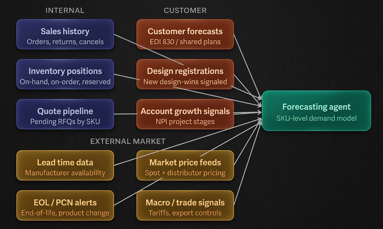
The internal signals are table stakes — every distributor has order history. What separates a good forecasting agent from a basic one is the customer signals layer. The most valuable of these is design registration data: when a customer registers a design win (telling you “I’m designing your component into a new product”), that is a leading indicator of future demand 6–18 months out — long before any purchase order is placed. A good agent correlates past design registrations with eventual order volumes to build a conversion model.
The external market signals are where the agent becomes genuinely unusual as a piece of software. It needs to be reading manufacturer lead time feeds (Octopart, SiliconExpert, direct API feeds from manufacturers like TI or NXP), parsing product change notices (PCNs) and end-of-life announcements, and monitoring trade policy news that could signal component restrictions.
How the model actually works
There’s no single model here — it’s a layered ensemble that combines several approaches.
The base layer is a classical time-series model (ARIMA, ETS, or Prophet depending on the SKU’s history length and seasonality pattern) that captures the trend and any cyclical patterns in order history. This works fine for stable, mature SKUs with years of data.
On top of that sits an ML layer — typically gradient boosting (XGBoost or LightGBM) — that takes the time-series forecast and adjusts it using all the contextual signals: customer pipeline data, lead time changes, market price signals. This is where the “why is demand about to spike” reasoning happens.
The third layer is the LLM reasoning layer — the “agent” part. This is what takes structured forecast outputs and applies judgment: “Customer X has a design win coming, but their NPI project is 3 months behind schedule, so I should delay the demand curve forward.” Or: “There’s a tariff change incoming that will likely cause customers to pull demand forward — I should front-load my inventory position.” This kind of contextual reasoning is where a pure ML model falls flat and where LLM-based agents add real value.
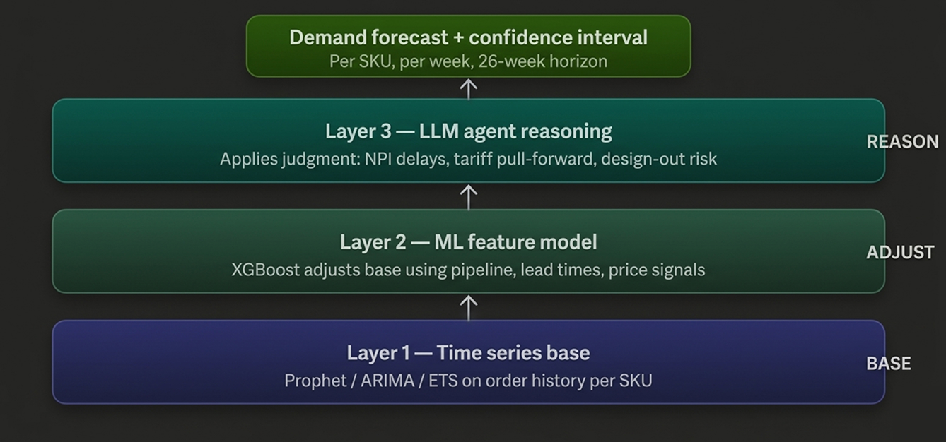
The agent doesn’t just output a number — it outputs a forecast per SKU per week across a rolling 26-week horizon (roughly one to two lead times out), with a confidence interval. High-confidence forecasts drive automated replenishment. Low-confidence forecasts get flagged for a human buyer to review.
The outputs and what they trigger
The forecast feeds three downstream processes directly:
The auto-replenishment agent (which we covered in the agent map) consumes the forecast and converts it into purchase order recommendations. The key parameter it receives is not just “expected demand” but also the confidence interval — a tight forecast with high confidence justifies lean inventory; a wide uncertain forecast justifies safety stock.
The obsolescence risk agent uses the forecast to identify SKUs where projected demand is declining faster than current inventory levels will clear. If the model predicts that demand for a particular FPGA will drop 60% over the next 6 months — because a newer generation is being designed in — the obsolescence agent can flag that you need to liquidate existing stock now, before it becomes unsellable.
The dynamic pricing agent uses forecast vs. inventory position to adjust sell prices. If you’re forecasting a supply shortage (lead times extending, demand steady), the agent can recommend holding price or even pricing up. If you’re sitting on excess inventory with declining demand, it recommends margin compression to accelerate turnover.
What makes a good vs. mediocre implementation
The difference between a forecasting agent that actually works in electronics distribution and one that doesn’t comes down to a few specific things.
SKU granularity is critical. Many distributors make the mistake of forecasting at the product family or category level. Electronics demand is highly SKU-specific — a particular package variant or temperature grade of a chip can have completely different demand dynamics than its sibling. The agent needs per-SKU, per-customer-segment forecasts, not rolled-up category forecasts.
Handling new SKUs is hard. By definition, a new product has no order history. The agent needs to cold-start by finding analogue SKUs — similar components from the same manufacturer, same application, similar price point — and borrowing their demand patterns. A good agent builds a SKU similarity model specifically for this.
Forecast explainability matters more than accuracy alone. A buyer who doesn’t understand why the agent is recommending 500 units of a sensor will override it. The LLM layer is genuinely valuable here because it can generate a natural-language rationale: “Forecast is 480 units over 12 weeks. Primary driver is the design-win registered by Acme Corp in January, plus seasonal uptick consistent with Q4 product launches in automotive. Confidence: medium — NPI project status unconfirmed.”
Finally, the feedback loop is what separates a static model from an improving agent. Every week, actual orders come in and get compared against the forecast. The agent should be continuously recalibrating — updating its weights, flagging which customer segments it is systematically over- or under-forecasting, and surfacing those patterns back to the buyer team as learnings.
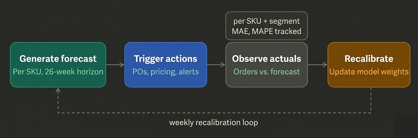
The recalibration loop is what turns this from a one-time analytics project into a compound-improving agent. Each week the model gets sharper — especially for the harder edge cases like new-product ramps and end-of-life rundowns.


There are no comments yet.